Simple Limber Example

A simple example showing how to apply the Limber model to correct for Limb darkening in a small SST/CRISP image. This data is loaded using astropy.fits, but crispy could be used too.

import matplotlib.pyplot as plt
import numpy as np
from astropy.io import fits
from smug.limber_adapter import LimberAdapter
from smug.limber_model import model_params, pretrained_limber

Load the Ca 8542 Angstrom data

im = fits.open("../tests/mini_crisp_l2_20140906_152724_8542_r00459.fits")

Load pretrained limber network

line = "CaII8542"
model = pretrained_limber(line)

Downloading: "https://www.astro.gla.ac.uk/users/USER-MANAGED/solar_model_weights/Limber_CaII8542_1.0.0.pth.tar" to /home/runner/.cache/torch/hub/checkpoints/Limber_CaII8542_1.0.0.pth.tar

  0%|          | 0.00/77.7M [00:00<?, ?B/s]
  0%|          | 32.0k/77.7M [00:00<04:52, 278kB/s]
  0%|          | 64.0k/77.7M [00:00<04:54, 277kB/s]
  0%|          | 96.0k/77.7M [00:00<04:53, 277kB/s]
  0%|          | 144k/77.7M [00:00<04:04, 332kB/s]
  0%|          | 208k/77.7M [00:00<03:16, 413kB/s]
  0%|          | 288k/77.7M [00:00<02:39, 508kB/s]
  0%|          | 384k/77.7M [00:00<02:11, 615kB/s]
  1%|          | 496k/77.7M [00:00<01:51, 729kB/s]
  1%|          | 656k/77.7M [00:01<01:26, 935kB/s]
  1%|1         | 848k/77.7M [00:01<01:09, 1.16MB/s]
  1%|1         | 1.09M/77.7M [00:01<00:52, 1.53MB/s]
  2%|1         | 1.42M/77.7M [00:01<00:40, 1.95MB/s]
  2%|2         | 1.86M/77.7M [00:01<00:31, 2.54MB/s]
  3%|3         | 2.41M/77.7M [00:01<00:24, 3.23MB/s]
  4%|3         | 3.03M/77.7M [00:01<00:19, 3.93MB/s]
  5%|4         | 3.80M/77.7M [00:01<00:16, 4.79MB/s]
  6%|6         | 4.70M/77.7M [00:02<00:13, 5.77MB/s]
  7%|7         | 5.77M/77.7M [00:02<00:10, 6.87MB/s]
  9%|9         | 7.09M/77.7M [00:02<00:08, 8.34MB/s]
 11%|#1        | 8.69M/77.7M [00:02<00:07, 10.1MB/s]
 13%|#3        | 10.5M/77.7M [00:02<00:05, 11.8MB/s]
 16%|#5        | 12.2M/77.7M [00:02<00:05, 12.9MB/s]
 18%|#7        | 13.9M/77.7M [00:02<00:04, 13.6MB/s]
 20%|##        | 15.7M/77.7M [00:02<00:04, 14.2MB/s]
 22%|##2       | 17.4M/77.7M [00:02<00:04, 14.6MB/s]
 25%|##4       | 19.2M/77.7M [00:03<00:04, 14.9MB/s]
 27%|##6       | 20.9M/77.7M [00:03<00:03, 15.0MB/s]
 29%|##9       | 22.6M/77.7M [00:03<00:03, 15.1MB/s]
 31%|###1      | 24.3M/77.7M [00:03<00:03, 15.2MB/s]
 34%|###3      | 26.1M/77.7M [00:03<00:03, 15.2MB/s]
 36%|###5      | 27.8M/77.7M [00:03<00:03, 15.3MB/s]
 38%|###8      | 29.6M/77.7M [00:03<00:03, 15.4MB/s]
 40%|####      | 31.3M/77.7M [00:03<00:03, 15.5MB/s]
 43%|####2     | 33.1M/77.7M [00:04<00:03, 15.4MB/s]
 45%|####4     | 34.8M/77.7M [00:04<00:02, 15.4MB/s]
 47%|####6     | 36.5M/77.7M [00:04<00:02, 15.4MB/s]
 49%|####9     | 38.3M/77.7M [00:04<00:02, 15.5MB/s]
 51%|#####1    | 40.0M/77.7M [00:04<00:02, 15.4MB/s]
 54%|#####3    | 41.8M/77.7M [00:04<00:02, 15.3MB/s]
 56%|#####5    | 43.5M/77.7M [00:04<00:02, 15.3MB/s]
 58%|#####8    | 45.2M/77.7M [00:04<00:02, 15.4MB/s]
 60%|######    | 47.0M/77.7M [00:04<00:02, 15.5MB/s]
 63%|######2   | 48.8M/77.7M [00:05<00:01, 15.5MB/s]
 65%|######4   | 50.5M/77.7M [00:05<00:01, 15.5MB/s]
 67%|######7   | 52.3M/77.7M [00:05<00:01, 15.6MB/s]
 69%|######9   | 54.0M/77.7M [00:05<00:01, 15.5MB/s]
 72%|#######1  | 55.7M/77.7M [00:05<00:01, 15.4MB/s]
 74%|#######3  | 57.5M/77.7M [00:05<00:01, 15.4MB/s]
 76%|#######6  | 59.2M/77.7M [00:05<00:01, 15.4MB/s]
 78%|#######8  | 61.0M/77.7M [00:05<00:01, 15.4MB/s]
 81%|########  | 62.7M/77.7M [00:06<00:01, 15.5MB/s]
 83%|########2 | 64.4M/77.7M [00:06<00:00, 15.5MB/s]
 85%|########5 | 66.2M/77.7M [00:06<00:00, 15.4MB/s]
 87%|########7 | 67.9M/77.7M [00:06<00:00, 15.4MB/s]
 90%|########9 | 69.6M/77.7M [00:06<00:00, 15.4MB/s]
 92%|#########1| 71.4M/77.7M [00:06<00:00, 15.4MB/s]
 94%|#########3| 73.1M/77.7M [00:06<00:00, 15.3MB/s]
 96%|#########6| 74.8M/77.7M [00:06<00:00, 15.4MB/s]
 99%|#########8| 76.6M/77.7M [00:06<00:00, 15.5MB/s]
100%|##########| 77.7M/77.7M [00:06<00:00, 11.6MB/s]

Compute wavelength grid used in Limber model from provided data, and construct Adapter.

grid = np.linspace(
    -model_params[line]["half_width"],
    model_params[line]["half_width"],
    model.size - 1,
)
limber_ca = LimberAdapter(model, grid)

Load wavelengths present in data file.

central_wavelength = np.median(im[1].data)
data_wavelength = im[1].data - central_wavelength

Run the network to reproject the data

out = limber_ca.reproject_data(
    im[0].data.astype("<f4"),
    data_wavelength,
    mu_observed=0.565,
    reconstruct_original_shape=False,
)

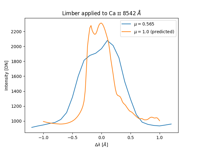
Plot the output for a pixel, note the swapped indexing as we set reconstruct_original_shape to False.

idx = 8
a = im[0].data.astype("<f4")
b = out
plt.plot(data_wavelength, a[:, idx, idx], label=r"$\mu=0.565$")
plt.plot(grid, b[idx, idx, 1:], label=r"$\mu=1.0$ (predicted)")
plt.xlabel(r"$\Delta\lambda$ [$\AA$]")
plt.ylabel("Intensity [DN]")
plt.title("Limber applied to Ca ɪɪ 8542 $\AA$")
plt.legend()
plt.show()